https:///weradocs/Wera_setup.shtml Last update:

WERA HF Radar Set-Up

Compiled by Yves Barbin / LSEET and Klaus-Werner Gurgel / Uni HH

1. Check Configuration and Installed Software Packages

  1. The CL7 (real time driving machine) and the Linux PC configurations have already been done
    (e.g. at the delivery by HELZEL Messtechnik). Check at the WERA Linux PC Configuration.
  2. Also check if all the archive files had been expanded and installed in the correct directories.
    The list of files is on the WERA HF Radar Software table, see webpage
    https://ifmaxp1.ifm.uni-hamburg.de/weradocs/Software.shtml.

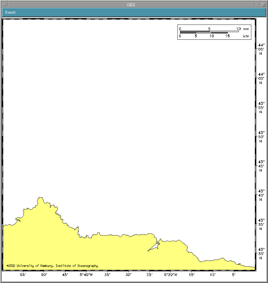
    For instance, Plott_UV needs access coast line data. These have been reformatted
    from a data set located at the University of Hawaii and are included in the
    coastlines_20020228.tar.gz archive.
2. Sites Selection Criteria

  1. Geometry and sea area coverage, use topographical or nautical map for initial selection and getting the site coordinates.
  2. Access (truck, crane, etc.) to the site and safety against vandalism.
  3. Ensure electrical power and data communication. Communication through a TCP/IP link; remote control and data transfer can be done. The Telemetry is possible at different levels ( type of results), which impacts on the link data rate and size of data file. Look at the Data Formats Section for information on how to calculate the size.
  4. Required Authorizations
    1. Installation:
      Area environmental issues, owner of the ground, the mayor, and who ever wants to be asked.
    2. Transmit license:
      Depends on the country and on the required range (radar frequency) and resolution (bandwidth), remark:
      A Joint Committee for Oceanography and Marine Meteorology (JCOMM) initiative regarding frequency allocation for HF radars is planned to be addressed to the ITU; Peter Dexter of JCOMM is to receive inputs from Klaus-Werner Gurgel. Users list of relevant persons in this area: K.-W. Gurgel, Lucy Wyatt, Mal Heron, Stuart Anderson, Don Barrick, Yves Barbin..... Initiative has to be pushed foreward.

3. Site Simulation

(In the following sections the /home/wera/ directory is quoted as ~/)
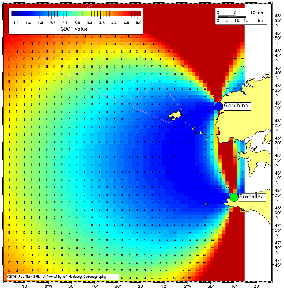
You now have the option to simulate the area covered by the radars and calculate the spatial distribution of errors (GDOP). Note that two or more sites have to be defined to calculate the GDOP:
  1. Edit the ~/etc/params.cfg and fill in the values documented for Plott_UV
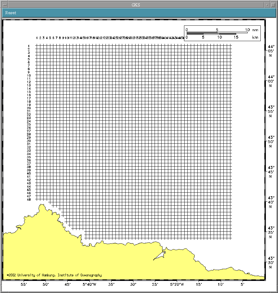
  2. Create a measurement grid by running ~/Fortran/Make_Grid
    Enter grid spacing and upper left corner when requested by Make_Grid.
    The number of grid points and the name of the grid file are taken from ~/etc/params.cfg
  3. Set WRITE_GDOP in ~/etc/params.cfg to .true. and run ~/Fortran/rad2uv once.
  4. Reset WRITE_GDOP in ~/etc/params.cfg to .false.
  5. Run ~/Fortran/Plott_UV and select one of the options -d=0     -d=1     -d=2     -d=3 .

4. Install the WERA

  1. Delivery and installation of container or radar housing, connection of electrical power. Take care of correct cooling of the rack modules.
  2. Connection of all WERA components (rack) inside the container.
  3. Switch on all the rack to allow warm up half a day, at least some hours to have a constant temperature (no dummy load required).
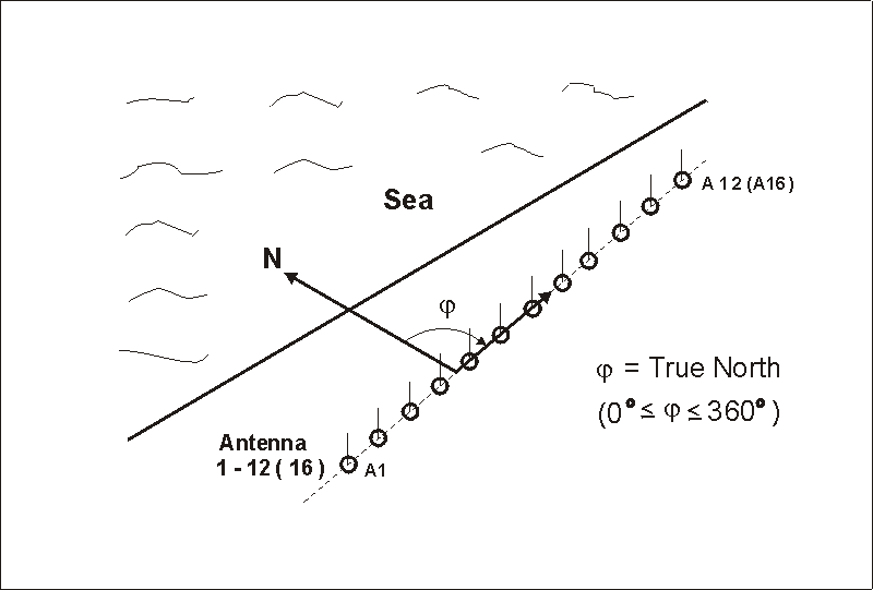
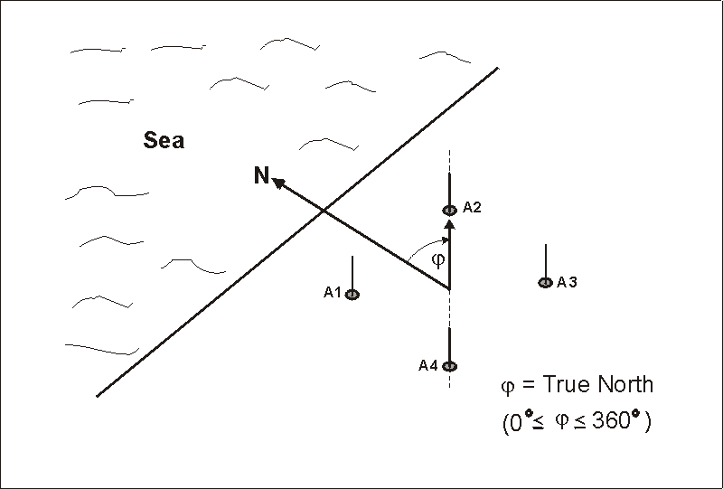
  4. Install the receive antenna array and measure "True North" for the linear array or for the square array.
  5. Install the transmit antenna array with phasing cables and power amplifier (PA).
  6. Install the transmit coax and power cables from the container to the PA.
  7. Fill in the WeraDesk parameters as described in the WeraDesk User Guide , e.g. radar working frequency, Lat/Lon of the site, True North of the receive antenna.

5. WERA Calibration

  1. Install the RX coaxial cables, connect them to the WERA receiver rack inside the container, eventually through short cables and spark arrestors, lay them down in the field towards the receiving antennas, connect all the "antenna" ends of the cables to the Calibration Box and connect the "Calibration Box" center to the radar rack transmit output through a step attenuator using an additional (long) cable.
  2. Connect one receiver output (e.g. antenna 1) to an x-y scope, select 'Test Calibration' and '80 Hz' offset from WeraDesk, and adjust the tx power with the step attenuator to give a circle of ~+/-8 Volts on the scope. Once the adjustment is done, select 'Test Stop' from WeraDesk.
  3. Reconnect the ADC to the receiver output, select '1024 samples', radar frequency, chirp length etc., select 'Calibration' from WeraDesk.
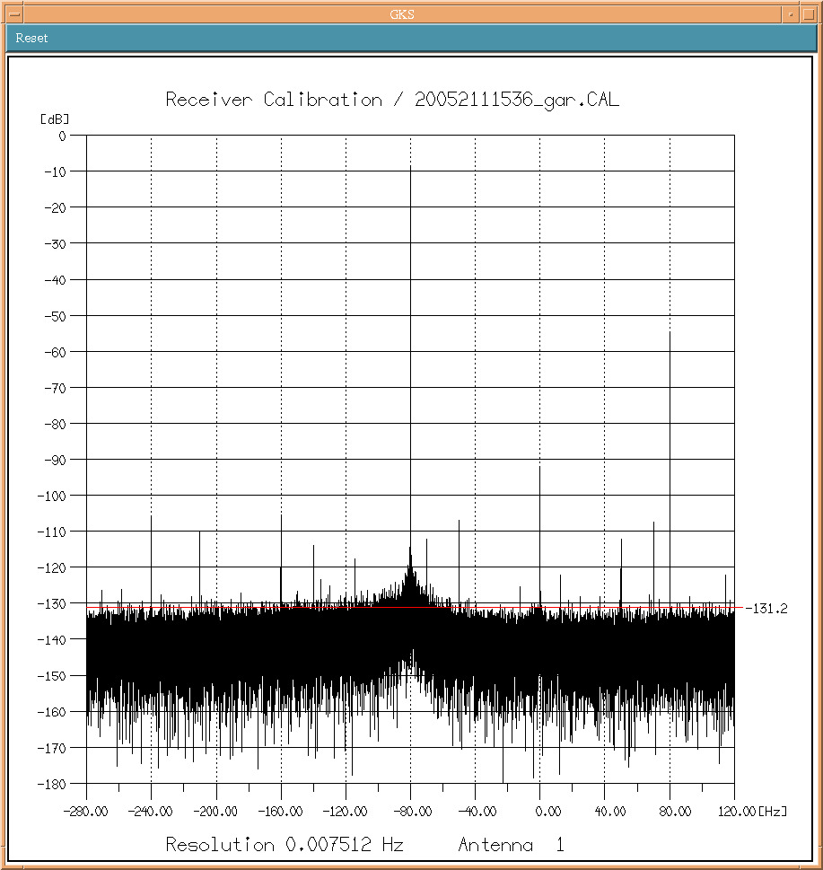
  4. Run three calibration measurements, process them by ~/Fortran/ Plott_WERA_Cal_lsq. Check if the phases and amplitudes given by Plott_WERA_Cal_lsq do not differ more than 1% between the measurements. Also check if the spectra give results similar to this example.
  5. Copy the calibration data file which best reflect the average values to ~/etc/calibration.wera as instructed by Plott_WERA_Cal_lsq.
  6. Remark: Instead of (4) you might use the 'Full Calibration' mode from WeraDesk V2.1.5 . This gives the complete characteristics (amplitude and phase) for all range cells and replaces the 'WERA Gain Ramp' (cf. the file ~/etc/wera_gain.dat) which has been measured with just one sample receiver.
    Caution - it takes about 4 hours to complete the 'Full Calibration'.

6. Running a single acquisition as a test

  1. Connect the coax cable running to the PA through a step attenuator to the WERA controller's TX output. Set that attenuator to 30 dB.
  2. Insert 10dB attenuation inside the PA at the PA input, connect a power meter (and a dummy load or antenna) to one of the 4 PA outputs.
  3. Select 'Test Calibration' and '80 Hz' offset from WeraDesk and adjust the PA HF output power with the step attenuator inside the container to give about 7.5 watts at the power meter (or the green LED inside the PA shining). If you use very long cables, you might need to remove the 10 dB inside the PA. Once the adjustment is done, select 'Test Stop' from WeraDesk. Note the value given by the step attenuator; this is the lowest attenuation you can use to prevent overdriving the PA.
  4. Remove the antenna 1 cable from the "Calibration Box", connect to antenna 1 now.
  5. Connect antenna 1 receiver output to an x-y scope, select 'Test Calibration' and '80 Hz' offset from WeraDesk, and adjust the step attenuator to give a circle of ~+/-8 Volts on the scope. Note the value of the step attenuator in a table for antenna 1.
  6. Repeat the last two steps for all the other antennas. Always note the value given by the step attenuator. By using this step-by-step connection of the antennas, you can identify any misconnection of antennas/cables/receivers.
  7. When finished with all antennas select 'Test Stop' and '0 Hz' offset. Select the highest attenuation value from the table just noted, subtract 10dB and compare that value to the attenuation needed for full PA power. Use the higher one of these two values during operation of the system. You may replace the step attenuator by a fixed one.
  8. Select 'Single Acquisition' and '2048 samples' from WeraDesk, start a measurement.
  9. Run Plott_WERA_Sort_RCs_Gain to check for sea echos (Bragg lines). If you have installed a linear array, you might want to form beams to look at specific directions using Plott_WERA_Sort_RCs_Beam instead. This should be enough for a short test. You can also process radial components of the surface current form a linear array (beam forming) by using
    1. wera16_grid, wera16_spec_rad, and Plott_UV
    2. wera16_beam, and Plott_UV
    or from a square array (direction finding) by using
    1. wera4_dir, and Plott_UV

Comments to: gurgel@ifm.uni-hamburg.de (Klaus-Werner Gurgel)